If you have ever used a GPS to avoid traffic, you already intuitively understand the fundamental problem of computer networks. When you send a message, it needs to traverse a “web” of routers to reach its destination.
But how do these devices decide where to go? Do they choose the path with the fewest cables? The fastest one? The cheapest one?
Today, we will dive into the theory behind Shortest Path Routing and understand the legendary Dijkstra’s algorithm, essential for any computer science student or network enthusiast.
1. The Treasure Map: Modeling the Network
Before we talk about algorithms, we need to visualize the network. Imagine the internet as a large graph:
- Nodes: Represent the routers.
- Links (Arcs): Represent the communication lines (cables, fiber, radio).

The goal of a routing algorithm is simple: look at this map and trace the optimal route between two points, even if the local router doesn’t know all the tiny details of the global network.
2. What Does “Shortest” Mean?
Here’s the catch. In the physical world, “short” usually means distance in kilometers. In networks, the answer is: it depends.
We can measure the “cost” of a path in several ways:
- Number of Hops: How many routers do we cross? If path ABC and ABE have the same number of edges, they are “equal” in this metric.
- Physical Distance: Actual kilometers of cable.
- Speed and Performance: This is where it gets interesting. We can label the arcs based on transmission delay, bandwidth (internet speed), financial cost, or average traffic.
Bottom Line: The “shortest” path for the algorithm might actually be the “fastest” or “least congested” path, depending on how we configure the weights (labels) of each connection.
3. Dijkstra’s Algorithm: The Star of the Show
Developed by Edsger W. Dijkstra in 1959, this algorithm is the basis for calculating routes in graphs. Its big idea is to find the best path from an origin to all other destinations in the network.
How it Works (Simplified Step-by-Step):
Imagine you are at router A and want to get to D.

- The Beginning: Since we don’t know the network yet, we assume the distance to all nodes is infinite, except for ourselves (which is zero).
- Tentative vs. Permanent Labels:
- Each node gets a label indicating the known distance to it.
- Initially, all are tentative (meaning, “this is the best path for now, but I might find a better one”).
- When we are absolutely sure there is no better path to that node, we make the label permanent.
- The Exploration (Greedy):
- You look at the neighbors of the current node.
- Calculate the cost to reach them. If the new cost is lower than what was noted there, you update the label.
- The Key Move: Among all the tentative nodes on the entire map, you choose the one with the lowest value and make it permanent. This node becomes the new starting point for the next round.
Why does this work?
It’s a logical question. If you chose node E to make permanent because it had the lowest tentative distance of all, it is impossible for a shorter path to exist passing through a distant node Z.
If Z offered a shortcut, the distance to Z would be less than to E, and we would have chosen Z first! (This assumes there are no negative distances in the network).
Implementation Curiosity: When programming this, we usually keep the “predecessor” node (where we came from). In the end, to show the route from A to Z, the computer reads backwards (Z, coming from Y, coming from X…) and reverses the list at the end to present the correct path.
4. Theory vs. Reality: The Sink Tree
When we calculate the optimal routes from all places to a single destination, we form a figure called a Sink Tree.

- It’s a tree: It has no loops (cycles). This ensures that the packet doesn’t spin forever and arrives in a finite number of hops.
- Or a DAG: If there is a tie (two paths with exactly the same cost), and we allow the use of both, the structure becomes a Directed Acyclic Graph (DAG).
The Real World Challenge:
All of this works perfectly on paper. In practice, routers go down (“go offline”) and come back up. This creates confusion: one router might think the path is clear while another knows it has fallen.
This inconsistency is the great challenge for network engineers. Therefore, the Optimality Principle and Sink Trees mainly serve as a benchmark, a gold standard for measuring the efficiency of the protocols we use every day.
Conclusion
Routing is the glue that holds the Internet together. Algorithms like Dijkstra’s show us that to find the best path, we don’t need magic, but rather a consistent step-by-step method that evaluates the real cost of each connection.
Did you like the explanation? If you are a networking student, try drawing a simple graph and running Dijkstra’s algorithm by hand. It’s the best way to fix the concept!
See more:
Congestion Control in Networks: Optimizing Efficiency and Bandwidth Allocation
Tutorial: How to use WHOIS and RDAP
https://www.rfc-editor.org/rfc/rfc2676.txt

Juliana Mascarenhas
Data Scientist and Master in Computer Modeling by LNCC.
Computer Engineer

Email Server & Webmail Setup: Postfix, Dovecot, SnappyMail
Install Ubuntu Server 26 on VirtualBox (Step-by-Step)
How to Configure NAT in Packet Tracer (Step-by-Step)

Zabbix FIM: How to Setup File Integrity Monitoring
Configure DHCP in Packet Tracer: Server & Router Guide